Let’s jump to the good stuff: How hard is it to create a program that can acoustic fingerprint a television show? Can we identify the playback position of a video based on audio tracks? For this blog post I’ll use The Drew Carey Show, because it’s the only show of which I have multiple seasons.
Crash Course
Acoustic fingerprinting is when a condensed audio signal is used to identify a larger audio sample. In practice, this means that given a small clip of audio from a movie or tv show, I would like to be able to identify the playback location where the clip originated. The complication is that, while a clip and it’s origin may sound exactly the same to the human ear, their binary representations may differ to do encoding, compression, or recording artifacts.
When writing about acoustic fingerprinting, it’s implied that the solution implemented needs to scale. What makes this interesting is not being able to match one clip out of dozens of samples, but being able to match one clip out of millions or billions of samples. Efficiency of technique is also implied when writing about fingerprinting. It’s not useful to generate a fingerprint that reduces the possible matches from ten million to a million, but it is useful to reduce the possible matches from ten million to ten. Scale matters, and by-proxy, efficiency matters. While I’ll try to apply scale and efficiency to the techniques in this project, it’s a little out of scope to find and catalogue millions of samples for my tests. For now, a couple seasons of The Drew Carey Show will have to do.
How does Shazam do it?
Shazam does fingerprinting by looking at spectrographic peaks that are “chosen according amplitude, with the justification that the highest amplitude peaks are most likely to survive [sic] distortions…” By listening to a song and finding two spectrographic peaks in the song, the algorithm Shazam uses is able to narrow down the number of potential candidates considerably. This is roughly the method I’ll use: reducing the audio track to a series of spectrographic peaks, tagging the peaks, and associating timestamps with them.
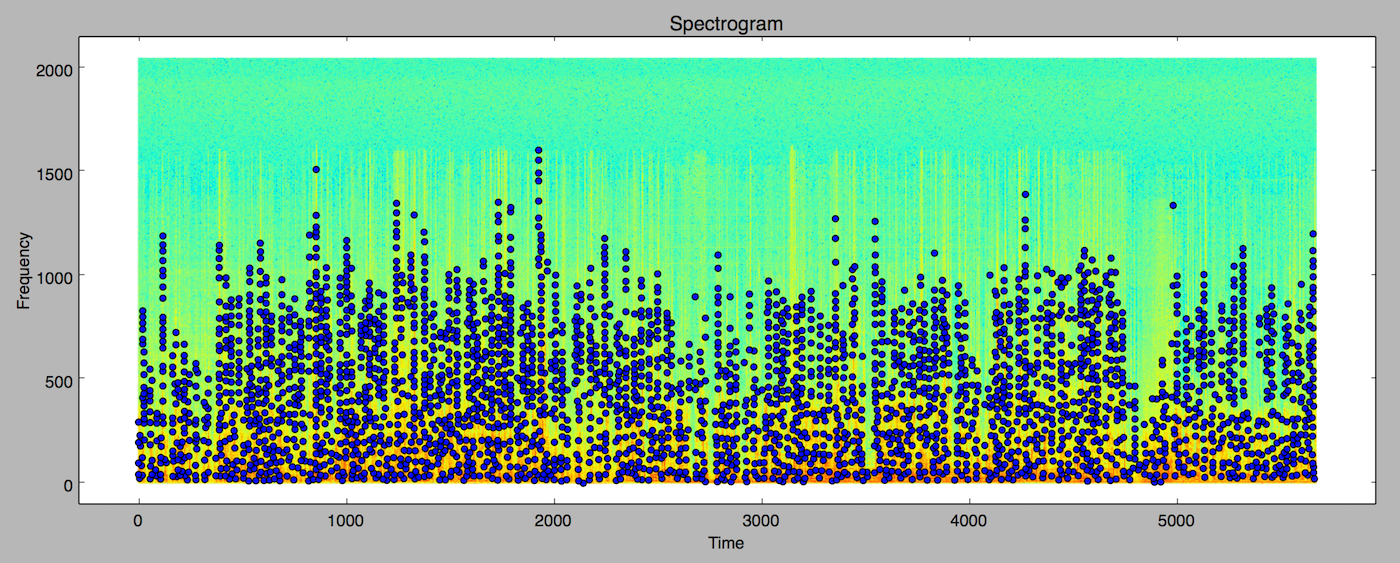
Once we have the audio separated from our video, and in a WAV file, it’s easier to work with. A WAV file is just a serialized bitstream of audio data, usually sampled at 44,100 Hz at 16 bits per sample. To put this into perspective, about a second of two channel audio is about 180Kb. To analyze the data, we can use matlab’s specgram library, which will sample the bitstream at a given window size using the Fast Fourier Transform (FFT) algorithm. FFT is the most common and one of the fastest ways of sampling a signal and breaking it down into its frequency components. So when we feed specgram the bitstream, we get an array of data back that represents the amplitude of frequency ranges of the signal at discrete points in time. Here’s what a WAV file for a couple of minutes of a movie looks like when we break to down by time (x axis), frequency (y axis) and amplitude (chromatic axis where green is low and red is high).
This type of data is really interesting, because when you visualize it like this, you get a sense that this could be basically any signal. Any type of signal that you get in wave format, you should be able to use signal analysis. I’d like to start a company called Sigint, and sell signal analysis tools on a large scale that can help spot patterns in large amounts of singal data.

The graph cuts off at ~2000 Hz, because human beings can’t hear anything higher than that. We can’t hear anything lower than 20 kHz, for that matter. If you look closely you’ll see that there doesn’t seem to be frequencies higher than 1600 Hz on the spectrograph. That’s because, at some point during the encoding process - when the video was being mastered, when it was compressed to DVD, when it was converted to AVI, or when it was converted to WAV - those frequencies were either compressed or eliminated. In the attempt to save disk space, someone decided that the viewer of the movie doesn’t care if there are sounds in the movie above 1600 Hz, and generally they’re right. This reduces the quality of the signal for our algorithm, but if those frequencies don’t exist in popular video formats, then our system will miss them anyway when put to use identifying a clip.
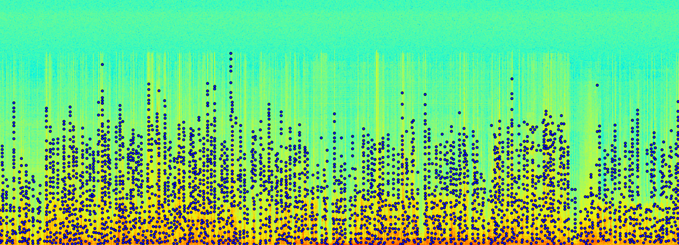
With the data in a format we can reason about, the next part of constructing a fingerprint involves figuring out the unique characteristics in the signal, in this case peaks. What defines a peak? We’ll define it as a given frequency range (R) going above a certain amplitude (A), with no other neighbors being higher for (N) neighbors. If we set R, A, or N too low, we’ll end up with so many peaks that when we use them to build a fingerprint, it will be too broad of an identifier. If we set these variables too high, then we’ll see fewer peaks, resulting in a fingerprint that will require too much capture time to match against. I’ll write about tuning these variables later. Here’s what it looks like when we scatterplot the peaks on top of the frequency data.
Fingerprinting and Indexing
Now that we have a list of peaks for a section of audio, we can uses these peaks to build our episode index. Peaks are just (time, frequency) pairs, e.g. (1197, 1941). Our index could be something like {frequency -> episode}. If we gather the frequency of enough peaks, we should be able to find which collection of frequencies exist sequentially in the same video. The performance of this technique isn’t going to be good though, because it would require multiple operations to lookup the video, and we would have to ensure the order when the query returns. At a minimum you would need to look up two peaks, but you could need many more to ensure that a match exists. What we can do instead is depend on time. If a frequency X is followed by frequency Y in a sample, and are separated by time T, we can use these three characteristics to build a hash, assuming that in any clip X, Y, and T will be roughly the same. For example, if we have two time-frequency pairs, our hash would be:
(941, 2247), (947, 907)
murmur3_hash("907:2247:6") = 2660468934
When we do a fingerprint lookup by hash, what we want back from the database is the episode and playhead position of that hash. Since two episodes could technically have the same hash and playhead position, we’ll use a compound index on hash, episode, and playhead position. This is pretty basic database stuff, so I won’t go into more detail.
Measuring and Testing
How do we know if this works? We can cut a 10 second clip from an episode and look for a match, which we’ll probably find; we’re running the same algorithm on the a subset of the bitstream we used to generate the fingerprint. The real test for fingerprinting is if the system is good at matching clips that are compressed, distorted, or otherwise altered from the original audio sample. To measure the effectiveness of the system more thoroughly I’ll randomly select 10 second clips from all of the episode we fingerprinted. I’ll then generate several distorted versions of each one:
- Light Background Noise (LBN): Equivalent of a coffee shop.
- Medium Background Noise (MBN): Equivalent of a quiet bar.
- Heavy Background Noise (HBN): Equivalent of a loud bar.
These are crude substitutes for recording actual clips in real watching environment where room acoustics, compression, distortions, and recording artifacts of any kind might disrupt the effectiveness of our algorithm, but they should give us a general sense of how well it would work in a likely application.
To ensure that our system isn’t finding patterns where none exist, I’ll also run these tests for clips from episodes that we did not fingerprint and load into the database. After all, if our system is able to match all of our loaded clips, but misses half of the non-loaded clips, then the system isn’t very good. The classification of outputs will follow positive-negative precision and recall:
- Positive Match: Correctly identified episode.
- False Positive Match: Incorrectly identified episode.
- Negative Match: Correctly rejected episode.
- False Negative Match: Incorrectly rejected episode.
In a nutshell, high precision means that most of the identified episodes were correct, and high recall means that many of the clips were correctly identified. If I had to choose one, I’d prefer high precision over high recall, because I don’t want to identify an episode and have it be the wrong one. Of course you could pick a low recall, and have high precision by limiting our system to only identifying clips when it’s 100% sure. What we’re looking for is a good balance of precision-recall.
Tuning the System
In the diagrams and discussion above, I’ve been assuming that our algorithm will have a roughly 10 second input sample to match against. Since we can’t always control how much data is given to our algorithm, I’ll run experiments using different sized clips, from 1 second all the way to 20 seconds. The system parameters I’ll tune are the fingerprint density (FD), the minimum amplitude (Amin), and the minimum peak range (Tmin).
Run 1
In the first run, I’ll start with FD = 0.8, Amin = 15, and Tmin = 15.
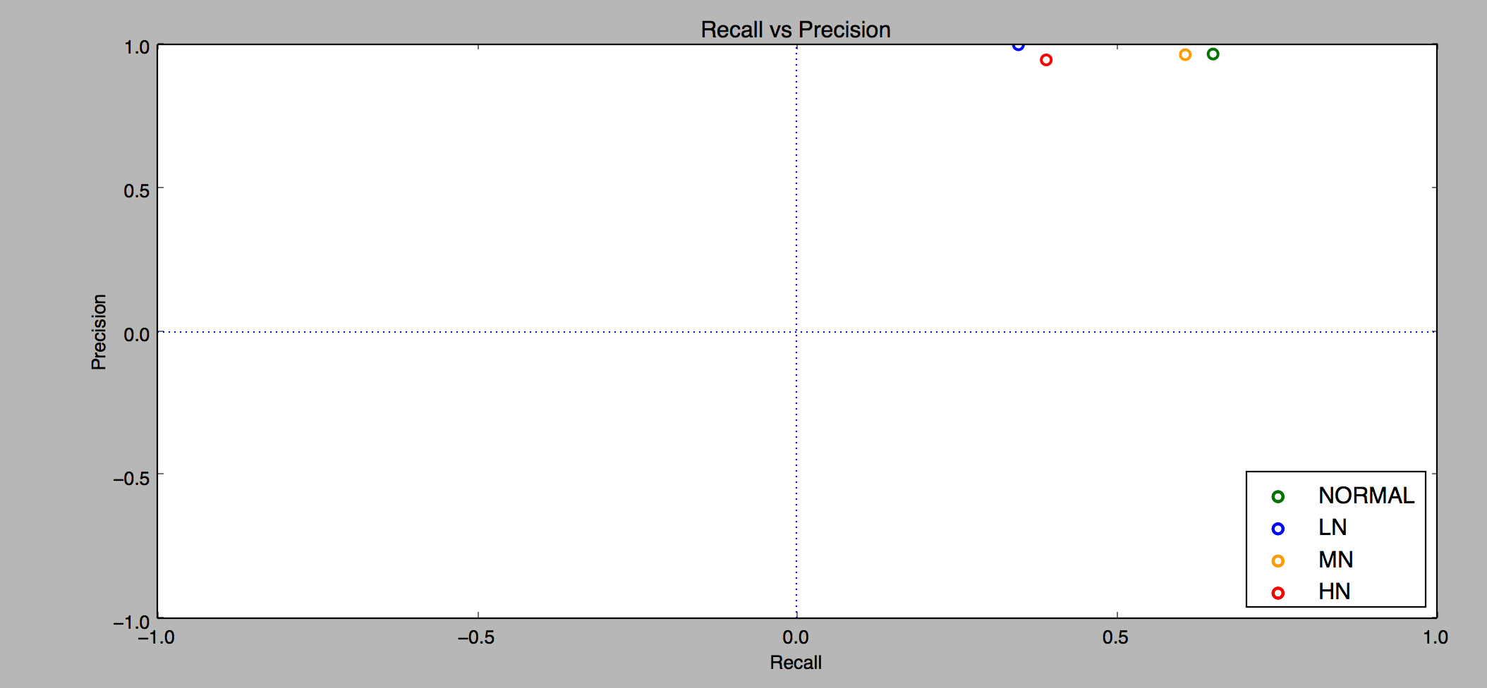
There’s a lot to unpack in this data, so let’s start with the first diagram. I ran the algorithm on 11 clean clips of length 1 through 20 seconds, and we can see that the precision stays at 100%, and the recall increases from 0% to 80%, maxing out at 15 second clips. We never reach a higher recall because with the current set of parameters we’ll never match 3 of the clips. The ones we couldn’t match all had quiet sections, with no discernible amplitude peaks. Given that there are no clear peaks in a quiet clip, our algorithm of matching sound peaks can’t work, which is fine. This is something we’d expect. No fingerprinting system works without some sort of baseline input.
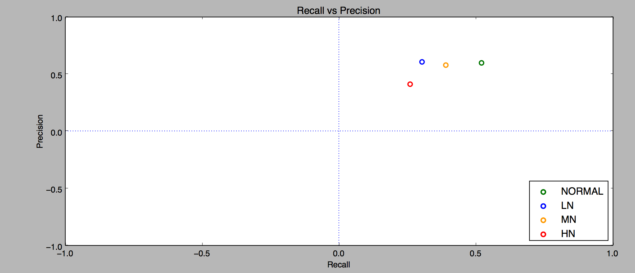
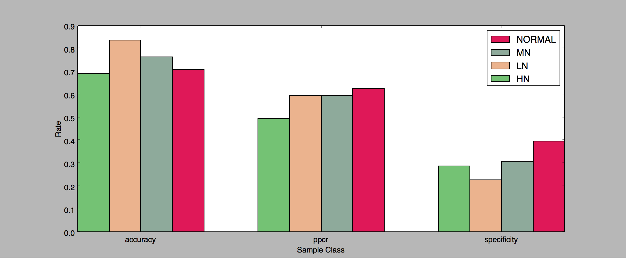
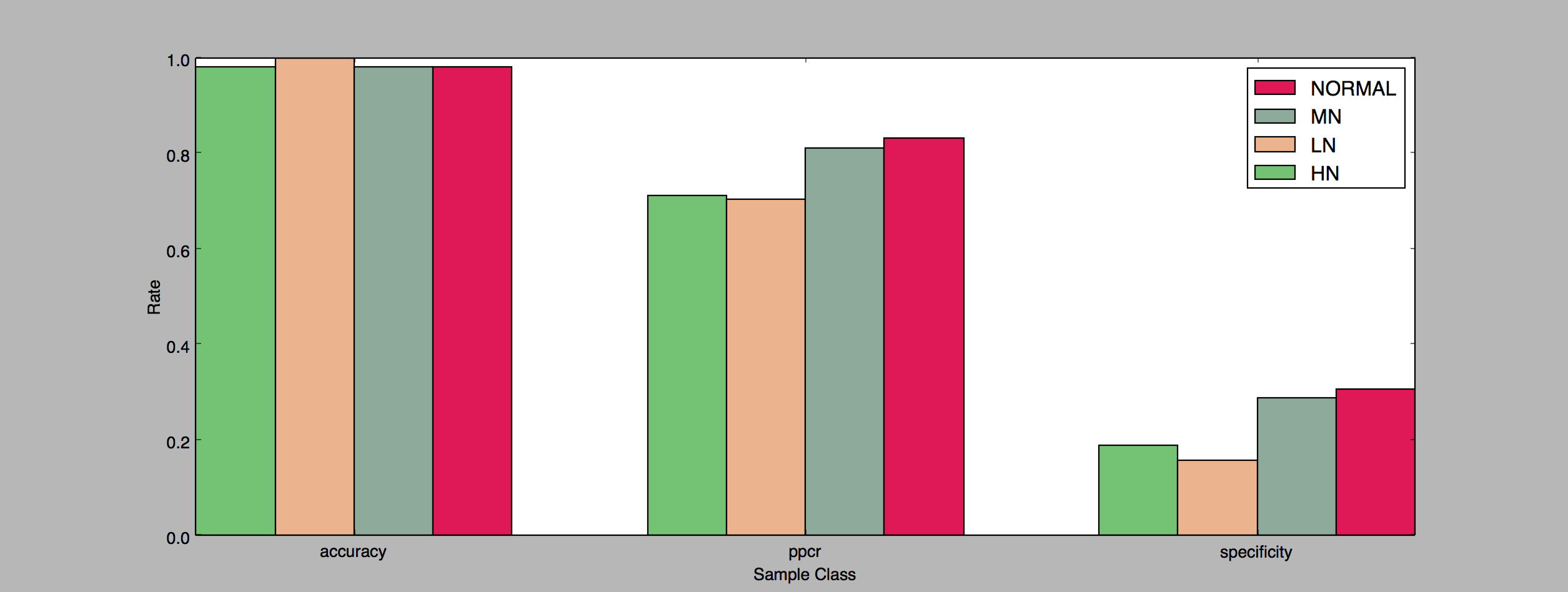
The second chart groups the results by clip length (5, 10, 15, and 20 seconds). The algorithm doesn’t do particularly well with the Light Background Noise, peaking at around 30% precision for the 15 second clips. With the current set of parameters it’s not able to match any clips with Medium or Heavy background noise.
Run 2
This time I’ll reduce FD = 0.5 (allowing for less dense fingerprints), increase Amin = 25 (requiring the peaks to be higher), and increase Tmin = 30 (requiring a longer period of time around a peak that doesn’t have higher neighbors).
With the new set of parameters, the clean recall climbs more slowly, only reaching 50% by the 5 second clip, and not plateauing like the first run. Unfortunately, the current set of parameters didn’t match any of the noisy clips. So I ran a couple more experiments before finding a set of parameters that matched noisy clips.
Run N
Well, to be honest, I lied. I ran the experiment about a hundred more times, on different data sets, with different parameters, and couldn’t get clean and noisy data to match at the same time. I tried the following: ignoring low frequencies (just background noise), ignoring high frequencies (reducing the fingerprint peaks to only the human voice range), or narrowing the fingerprint matching. Something more drastic was necessary.
So I began looking at the peaks. In the below image the peaks-fingerprints generated from the clip are red, and the fingerprint-peaks from the episode are green. The further away from one-another, the less likely they will be a match.
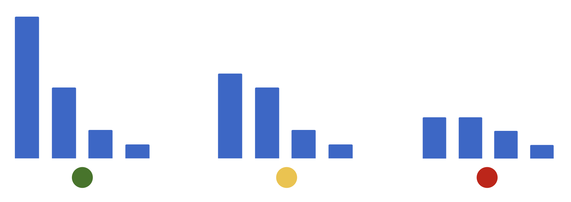
When the green peaks are close to the red peaks there is a match. Looking at the data, I was able to find clean clips that had matches with this data, and noisy clips that did not. As you can see, most of the fingerprints from the noisy clips are totally different. The background noise added to the clips changes the characteristics of the clip so much that it’s unlikely they’ll match. So the next approach I tried was to threshold the matches. As long as there were N fingerprints that matched, where N is a function of the clip length, the clip should be classified as a match.
Result
That did it! Once I calculated the probability of peak fingerprints matching, the clips were mostly correctly identified. With the right calibration, I can get 100% recall/precision on clean clips, 60-80% recall/precision on light-noise clips, 40-60% recall/precision on medium-noise clips, and 10-20% recall/precision on heavy-noise clips.
Folder Structure
The directory structure is like this:
/acousticfingerprint.py
/data
  /episodes
    /s1
      /e1.wav
      /e2.wav
      ...
    /s2
      /e1.wav
      /e2.wav
      ...
    ...
  /clips
    /s1_e1_13320.wav
    /s1_e2_107250.wav
    ...
    /s2_e21_38325.wav
    ...
Python Function
def find_2D_peaks(arr2D, amp_min=DEFAULT_AMP_MIN,
                  peak_range=DEFAULT_RANGE):
    struct = generate_binary_structure(2, 1)
    neighborhood = iterate_structure(struct, peak_range)
    local_max = maximum_filter(arr2D, footprint=neighborhood) == arr2D
    background = (arr2D == 0)
    eroded_background = binary_erosion(background,
                                       structure=neighborhood,
                                       border_value=1)
    detected_peaks = local_max - eroded_background
    amps = arr2D[detected_peaks]
    j, i = np.where(detected_peaks)
    amps = amps.flatten()
    peaks = zip(i, j, amps)
    peaks_filtered = [x for x in peaks if x[2] > amp_min]
    frequency_idx = [x[1] for x in peaks_filtered]
    time_idx = [x[0] for x in peaks_filtered]
    return zip(frequency_idx, time_idx)
I’d love to write more about this, but I’ve reached my time-limit. That’s all for now.